Simulation-based inference

After performing the inital dynamical systems analysis of a single frontostriatal circuit (i.e. only one cortex and striatum), we coupled two frontostriatal circuits : the ventromedial circuit composed of the orbitofrontal cortex (OFC) and the nucleus accumbens (NAcc), with the dorsolateral circuit composed of the lateral prefrontal cortex (LPFC) and the dorsal putamen (dPut).

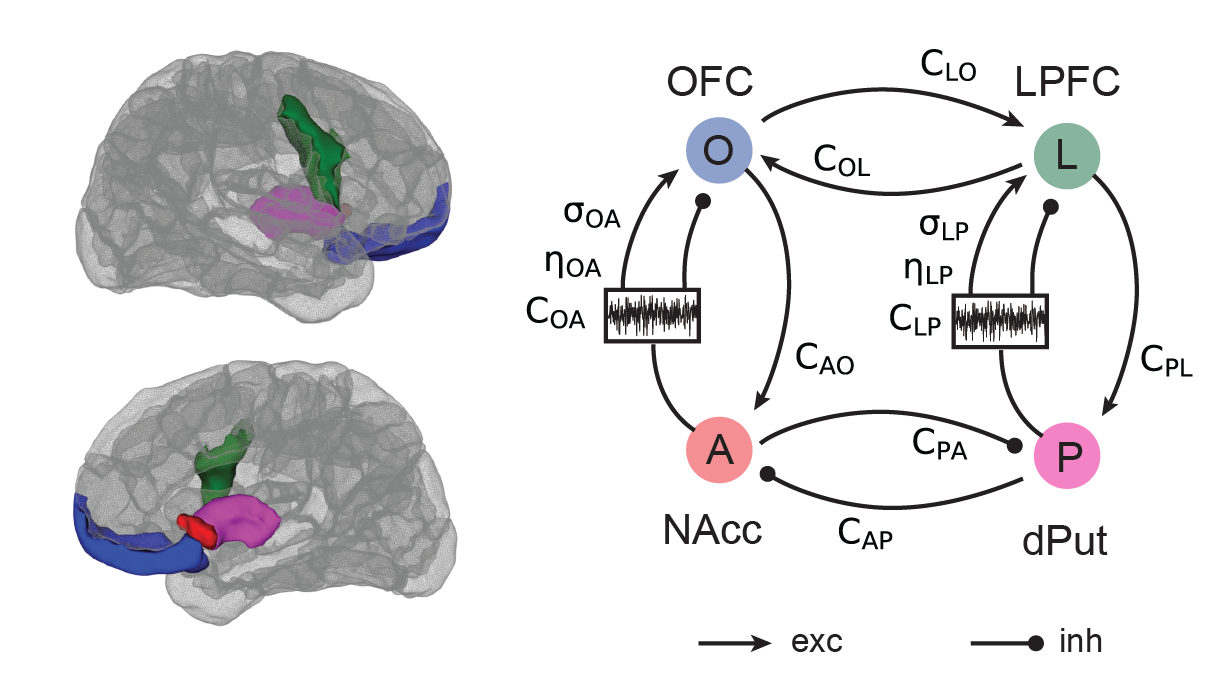
Illustration of the coupled ventromedial and dorsolateral frontostriatal circuits.

The dynamical systems analysis of this coupled system becomes untractable without making considerable simplifications or unreasonnable assumptions.

Instead, we exploited an optimization framework to find the parameter distributions underlying the dynamics of this model for healthy and OCD subjects.

Parameter optimization

We perform parameter optimization using Approximate Bayesian Computation with a Sequential Monte-Carlo algorithm (ABC-SMC) implemented in the pyABC toolbox (Klinger et al., 2022).

We exploited the computational power offered by our high-performance computing infrastructure by instanciating a REDIS server, which handled the I/O and provided a lightweight database accessible by the worker nodes. For more information, visit https://pyabc.readthedocs.io/en/latest/api/pyabc.sampler.html#pyabc.sampler.RedisEvalParallelSampler.

Once the server is set up, we instanciate and run the ABC-SMC, which is the core class of the toolbox: https://pyabc.readthedocs.io/en/latest/api/pyabc.inference.html

Each worker node is running simulations (Parent Processes) using parameters generated (by the Master process) and stored in the (REDIS) server.

Architecture of the parallel optimization.

OCD_modeling.mcmc.simulate_population_rww(params)

Run a pool of simulations and score their outputs.

As a design choice, the number of simulations per pool and the number of processes used in parallel are hard coded here in a Argparse.Namespace object which is propagated to the launcher.

Parameters:

params (dict) – Set of parameters are used to instanciate model.

Returns:

RMSE – Root Mean Square Error between the simulated pool (i.e. a “population cohort”) and the real data (either “controls” or “patients”).

Return type:

dict

The simulations are further parallelized across processes (Child Processes) within a single worker.

OCD_modeling.hpc.launch_pool_simulations(args)

Launch N simulations in parallel using a Pool Executor.

Parameters:

args (Argparse.Namespace) – Structure containing the information of the siumulation to be performed: model, simulation, control and BOLD parameters.

Returns:

sim_objs – Simulation objects after processing.

Return type:

list of OCD_modeling.models.ReducedWongWangOU

OCD_modeling.hpc.run_sim(model_pars, sim_pars, control_pars={}, bold_pars={})

Run a single simulation.

Parameters:

• model_pars (dict) – Model parameters (e.g. couplings, noise, external inputs, etc.)

• sim_pars (dict) – Simulation parameters (e.g. simulation time, reccording intervals, sampling frequency, etc.)

• control_pars (dict) – Control parameters. In case parameters needs to be manually updated throughout the simulation, provide the parameters’ timeseries here.

• bold_pars (dict) – BOLD parameters. Dictionary with keys t_range (the time range on which to compute the BOLD signal), and transient (the time to discard due to transient at hthe beginning on the convolution).

Returns:

rww_sim – Simulation object, containing raw and processed data (BOLD timeseries, functional connectivity, transitions).

Return type:

OCD_modeling.models.ReducedWongWangOU

History analysis

Once parameters have been optimized to fit empirical data, we can visualize the posterior distributions of model’s parameters.

OCD_modeling.mcmc.compute_kdes(histories, n_pts=100, args=None)

Computes Kernel Density Estimates (KDEs) of the posterior distributions of parameters.

Parameters:

• histories (dict) – Nested dictionnary of SQL alchemy history objects.

• n_pts (int) – Number of points used to estimate the probability density functions (PDFs).

• args (argparse.Namespace) – Extra options.

Returns:

• kdes (dict) – Nested dictiorany of KDEs and associated PDFs.

• cols (list) – List of parameters for which the KDEs were estimated.

OCD_modeling.mcmc.plot_kdes(kdes, cols, df_stats, df_real=[], df_pred=[], plot_args={'col_offset': 3, 'figsize': [10, 7], 'hist_alpha': 0.3, 'kde_alpha': 1, 'ncols': 5, 'nrows': 4, 'row_offset': 2, 'show_stars': True}, args=None)

Plot Kernel Density Estimates of posteriors (controls vs OCD)

Parameters:

• kdes (dict) – Kernel Density Estimates of parameters

• cols (list) – Model parameters

• df_stats (pandas.DataFrame) – Stastics for each parameter (healthy controls vs OCD patients)

• df_real (pandas.DataFrame) – (Optional) Synthetic data (observed)

• df_pred (pandas.DataFrame) – (Optional) Synthetic data (predicted)

• plot_args (dict) –

  Default options for plotting.

  nrows, ncols: number of rows and columns of the GridSpec object (grid of axes). row_offset, col_offset: shifts in rows and colums to let space for another plot. figsize: figure size. show_stars: show stars for statistical significant between controls and OCD. hist_alpha, kde_alpha: opacity of the histograms and kernel density estimates.

• args (argparse.Namespace) – (Optional) Extra arguments

Plotting Kernel Density Estimates (KDEs)

We perform statistical test on those posterior distribution to extract parameters differentiating OCD subjects from healthy controls.

OCD_modeling.mcmc.compute_stats(histories, args=None)

Computes the statistics of the optimization outcome, i.e. tests the posterior distributions (parameters) between controls and patients.

Parameters:

• histories (list) – Controls and patient pyABC history objects.

• args (argparse.Namespace) – Extra options

Returns:

df_stats – Statistics.

Return type:

pandas DataFrame

We can also verify the meta parameters of the optimizer. Weights distributions indicate whether the sampling at the different generations is using a large number of particles or only a few individuals of a population (indicative of degeneracy). Visualizing the error rate \(\epsilon\) indicates how far is the optimization from the target value and whether the optimization is still progressing or plateauing.

OCD_modeling.mcmc.plot_weights(histories, gs=None, nrows=None, ncols=None, row_offset=None, col_offset=None, args=None)

Plot evolution of weights across generations

Parameters:

• histories (list) – Optimization pyABC history objects (e.g. controls and patients)

• gs (matplotlib.GridSpec) – (optional) GridSpec object to draw the figure into.

• nrows (int) – number of rows/columns to make the grid.

• ncols (int) – number of rows/columns to make the grid.

• row_offset (int) – offsets to account for when some (top left) entries of the grid should be left empty.

• col_offset (int) – offsets to account for when some (top left) entries of the grid should be left empty.

• args (argparse.Namespace) – (optional) Extra arguments (e.g. for saving, etc).

OCD_modeling.mcmc.plot_epsilons(histories, ax=None, args=None)

Plot evolution of epsilons across generations

Parameters:

• histories (list) – Optimization pyABC history objects (e.g. controls and patients)

• ax (matplotlib.Axes) – (optional) Axis to draw the figure.

• args (argparse.Namespace) – (optional) Extra arguments (for saving, etc).

[A] Error rates (\(\epsilon\)) and [B] Weights \(\omega\) of the optimization (blue: contols; orange:OCD).

Synthetic dataset

We then generate new synthetic data using posterior distributions of parameters infered by the ABC-SMC algorithm.

OCD_modeling.mcmc.launch_sims_parallel(kdes, cols, test_param, args=None)

Run batched simulations from posterior inference in parallel:

Parameters:

• kdes (dict) – Kernel Density Estimates from optimization (structured as kdes[group][param])

• cols (list) – Parameters (columns) which draw samples from KDEs (otherwise default values are used)

• test_param (list) – Parameters for which the posterior is permuted for the virtual interventions.

• args (argparse.Namespace) – Extra arguments with options.

Return type:

None. Output of the simulations are written into the local SQLite database.

The distribution of functional connectivities across the frontostriatal system can be visualized and compared between empirical (observed) and simulated data.

OCD_modeling.mcmc.plot_fc_sim_vs_data(df_data, df_base, stats, axes=None, args=None)

Plot functional connectivity (Pearson correlation) across the frontostriatal regions of interests in empirical and simulated data.

Parameters:

• df_data (pandas.DataFrame) – Empirical data extracted from fMRI in OCD subjects and healthy controls.

• df_base (pandas.DataFrame) – Simulated data using parameters infered from posterior distributions (either only OCD parameters or only controls, no permutation to model virtual intervention).

• stats (dict) – (deprecated) Statistics within and between cohorts for both empirical and simulated data (deprecated since now stats are directly computed within plotting function).

• axes (list of matplotlib.Axes) – (optional) List of axes to plot data (if embedded in other figure, otherwise create new figure).

• args (argparse.Namespace) – (optional) Extra arguments (e.g. for saving, etc).

Functional connectivity patterns across the frontostriatal system in OCD subjects (orange) vs healthy controls (blue), from empirical (observed) and simulated data.

Model comparison

While the ABC-SMC optimization framework does incorporate Bayesian model selection during the optimization process, we sometimes want to compare the performance of different optimized models post-hoc.

This task simply involves computing the error between the synthetic data generated by each model and the empirical data that we are optimized against.

First, load the empirical and simulated datasets:

OCD_modeling.mcmc.load_empirical_data()

Load empirical dataset that we optimized against.

Returns:

df_data – Empirical dataset with subjects and functional connecticity (Pearson’s correlation) in each frontostriatal pathways.

Return type:

pandas.DataFrame

OCD_modeling.mcmc.load_simulations(args)

Load simulated inferences.

Parameters:

args (argparse.Namespace) – Dictionnary-like datastructure containing args.db_names argument which was enterred in command-line as a list of simulated dataset.

Returns:

out – List of pandas.DataFrame, each containing n simulations with functional connectivity in each frontostriatal pathway. (default n=1000)

Return type:

list

Then, compute and plot errors:

OCD_modeling.mcmc.compute_errors(df_sims, df_data, args)

Compute root-mean-square errors between empirical and simulated data in frontostriatal pathways functional connectivity.

This error takes the form of a distribution, i.e. with 1000 simulations grouped by cohorts of 50, it makes 20 error values.

Parameters:

• df_sims (pandas.DataFrame) – Simulated dataset.

• df_data (pandas.DataFrame) – Empirical dataset.

• args (argparse.Namespace) – Optional arguments.

Returns:

Distribution of errors in functinal connectivity space.

Return type:

pandas.DataFrame

OCD_modeling.mcmc.plot_errors(df_errors, args)

Box plot of inference error on frontostriatal functional connectivity

Parameters:

• df_errors (pandas.DataFrame) – Distributions of errors for each models to compare.

• args (argparse.Namespace) – Optional arguments, including args.model_tags that contains labels of model names for saving.

Error between simulated models (without thalamus nodes, N=4; with thalamus nodes, N=6) and empirical frontostriatal connectivity data.